Load mapped read-ends and generate a matrix

We read now each mapped read-ends in the map files and extact the ones that are uniquely mapped. For each of these uniquely mapped read-ends, we store: - The strand - The genomic location (most upstream position is reported for both sequences mapped in forward and reverse strand) - The chromosome - The sequence itself - The restriction enzyme fragment on which it is located

This information will be used to filter the reads and, finally, to construct the interaction matrix. Above we show the same analysis done for the fragment-based and iterative mapping strategies.

Extract uniquely mapped reads

# replicate and enzyme used
cell = 'mouse_B'  # or mouse_PSC
rep = 'rep1'  # or rep2

Note: the execution of this notebook should be repeated for each of the 4 replicates

Load genomic sequence to map restriction sites

from pytadbit.parsers.genome_parser import parse_fasta

genome_seq = parse_fasta('genome/Mus_musculus-GRCm38.p6/Mus_musculus-GRCm38.p6.fa')

Loading cached genome

from pytadbit.parsers.map_parser import parse_map

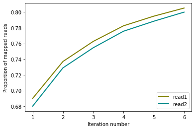
Iterative mapping results

In case we haven’t stored the location of each of the reads we could load them as follow:

maps1 = [('results/iterativ/{0}_{1}/01_mapping/mapped_{0}_{1}_r1/'
          '{0}_{1}_1.fastq_full_1-{2}.map').format(cell, rep, i)
         for i in range(25, 80, 10)]

maps2 = [('results/iterativ/{0}_{1}/01_mapping/mapped_{0}_{1}_r2/'
          '{0}_{1}_2.fastq_full_1-{2}.map').format(cell, rep, i)
         for i in range(25, 80, 10)]

Load all reads, and check if they are uniquely mapped. The Result is stored in two separate tab-separated-values (tsv) files that will contain the essential information of each read-end

! mkdir -p results/iterativ/$cell\_$rep/02_parsing

parse_map(maps1, maps2,
          'results/iterativ/{0}_{1}/02_parsing/reads1_{0}_{1}.tsv'.format(cell, rep),
          'results/iterativ/{0}_{1}/02_parsing/reads2_{0}_{1}.tsv'.format(cell, rep),
          genome_seq=genome_seq, re_name='MboI', verbose=True)

Searching and mapping RE sites to the reference genome
Found 6669655 RE sites
Loading read1
loading file: results/iterativ/mouse_B_rep1/01_mapping/mapped_mouse_B_rep1_r1/mouse_B_rep1_1.fastq_full_1-25.map
loading file: results/iterativ/mouse_B_rep1/01_mapping/mapped_mouse_B_rep1_r1/mouse_B_rep1_1.fastq_full_1-35.map
loading file: results/iterativ/mouse_B_rep1/01_mapping/mapped_mouse_B_rep1_r1/mouse_B_rep1_1.fastq_full_1-45.map
loading file: results/iterativ/mouse_B_rep1/01_mapping/mapped_mouse_B_rep1_r1/mouse_B_rep1_1.fastq_full_1-55.map
loading file: results/iterativ/mouse_B_rep1/01_mapping/mapped_mouse_B_rep1_r1/mouse_B_rep1_1.fastq_full_1-65.map
loading file: results/iterativ/mouse_B_rep1/01_mapping/mapped_mouse_B_rep1_r1/mouse_B_rep1_1.fastq_full_1-75.map
Merge sort....................................................................................
Getting Multiple contacts
Loading read2
loading file: results/iterativ/mouse_B_rep1/01_mapping/mapped_mouse_B_rep1_r2/mouse_B_rep1_2.fastq_full_1-25.map
loading file: results/iterativ/mouse_B_rep1/01_mapping/mapped_mouse_B_rep1_r2/mouse_B_rep1_2.fastq_full_1-35.map
loading file: results/iterativ/mouse_B_rep1/01_mapping/mapped_mouse_B_rep1_r2/mouse_B_rep1_2.fastq_full_1-45.map
loading file: results/iterativ/mouse_B_rep1/01_mapping/mapped_mouse_B_rep1_r2/mouse_B_rep1_2.fastq_full_1-55.map
loading file: results/iterativ/mouse_B_rep1/01_mapping/mapped_mouse_B_rep1_r2/mouse_B_rep1_2.fastq_full_1-65.map
loading file: results/iterativ/mouse_B_rep1/01_mapping/mapped_mouse_B_rep1_r2/mouse_B_rep1_2.fastq_full_1-75.map
Merge sort...................................................................................
Getting Multiple contacts

({0: {1: 69012817, 2: 4693142, 3: 2552881, 4: 1982032, 5: 1225598, 6: 1031718},
  1: {1: 68026433,
   2: 4866307,
   3: 2558036,
   4: 2103111,
   5: 1271540,
   6: 1153164}},
 {0: {0: 80498187}, 1: {0: 79978590}})

from pytadbit.mapping.analyze import plot_iterative_mapping

total_reads = 100000000

lengths = plot_iterative_mapping(
    'results/iterativ/{0}_{1}/02_parsing/reads1_{0}_{1}.tsv'.format(cell, rep),
    'results/iterativ/{0}_{1}/02_parsing/reads2_{0}_{1}.tsv'.format(cell, rep),
    total_reads)

Fragment-based mapping results

! mkdir -p results/fragment/$cell\_$rep/02_parsing

maps1 = [('results/fragment/{0}_{1}/01_mapping/mapped_{0}_{1}_r1/'
          '{0}_{1}_1.fastq_full_1-end.map').format(cell, rep),
         ('results/fragment/{0}_{1}/01_mapping/mapped_{0}_{1}_r1/'
          '{0}_{1}_1.fastq_frag_1-end.map').format(cell, rep)]

maps2 = [('results/fragment/{0}_{1}/01_mapping/mapped_{0}_{1}_r2/'
          '{0}_{1}_2.fastq_full_1-end.map').format(cell, rep),
         ('results/fragment/{0}_{1}/01_mapping/mapped_{0}_{1}_r2/'
          '{0}_{1}_2.fastq_frag_1-end.map').format(cell, rep)]

parse_map(maps1, maps2,
          'results/fragment/{0}_{1}/02_parsing/reads1_{0}_{1}.tsv'.format(cell, rep),
          'results/fragment/{0}_{1}/02_parsing/reads2_{0}_{1}.tsv'.format(cell, rep),
          genome_seq=genome_seq, re_name='MboI', verbose=True)

Searching and mapping RE sites to the reference genome
Found 6669655 RE sites
Loading read1
loading file: results/fragment/mouse_B_rep1/01_mapping/mapped_mouse_B_rep1_r1/mouse_B_rep1_1.fastq_full_1-end.map
loading file: results/fragment/mouse_B_rep1/01_mapping/mapped_mouse_B_rep1_r1/mouse_B_rep1_1.fastq_frag_1-end.map
Merge sort...........................................................................................
Getting Multiple contacts
Loading read2
loading file: results/fragment/mouse_B_rep1/01_mapping/mapped_mouse_B_rep1_r2/mouse_B_rep1_2.fastq_full_1-end.map
loading file: results/fragment/mouse_B_rep1/01_mapping/mapped_mouse_B_rep1_r2/mouse_B_rep1_2.fastq_frag_1-end.map
Merge sort........................................................................................
Getting Multiple contacts

({0: {1: 64750569, 2: 25664719}, 1: {1: 61548041, 2: 26467447}},
 {0: {1: 8157782, 0: 74098430, 2: 431}, 1: {0: 71100363, 1: 8456843, 2: 479}})

reads1 = 'results/fragment/{0}_{1}/02_parsing/reads1_{0}_{1}.tsv'.format(cell, rep)
reads2 = 'results/fragment/{0}_{1}/02_parsing/reads2_{0}_{1}.tsv'.format(cell, rep)

from pytadbit.mapping.analyze import plot_iterative_mapping

total_reads = 100000000

lengths = plot_iterative_mapping(reads1, reads2, total_reads)

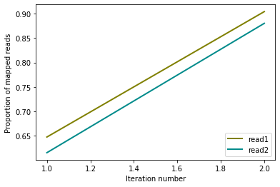
Note: From now on we are going to focus only on the results of thefragment based mapping.

Keep only uniquely mapped reads pairs

from pytadbit.mapping import get_intersection

! mkdir -p results/fragment/$cell\_$rep/03_filtering

reads = 'results/fragment/{0}_{1}/03_filtering/reads12_{0}_{1}.tsv'.format(cell, rep)

get_intersection(reads1, reads2, reads, verbose=True)

Getting intersection of reads 1 and reads 2:

  .......... .......... .......... .......... ..........     50 milion reads
  .......... .......... .......... .......... ...
Found 68707083 pair of reads mapping uniquely
Sorting each temporary file by genomic coordinate
    1025/1025 sorted files
Removing temporary files...

(68707083, {2: 9191166, 3: 154507, 4: 17})

Quality check of the Hi-C experiment

from pytadbit.mapping.analyze import plot_distance_vs_interactions

plot_distance_vs_interactions(reads, resolution=100000, max_diff=1000, show=True)

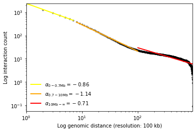
((-0.8597345093043444, 7.77896435141178, -0.9993659328855855),
 (-1.1357021175965485, 8.287957073239085, -0.9982246432365471),
 (-0.7085449034953684, 6.662855682899386, -0.8479147001712137))

According to the fractal globule model (Mirny, 2011) the slope between 700 kb and 10 Mb should be around -1 in log scale

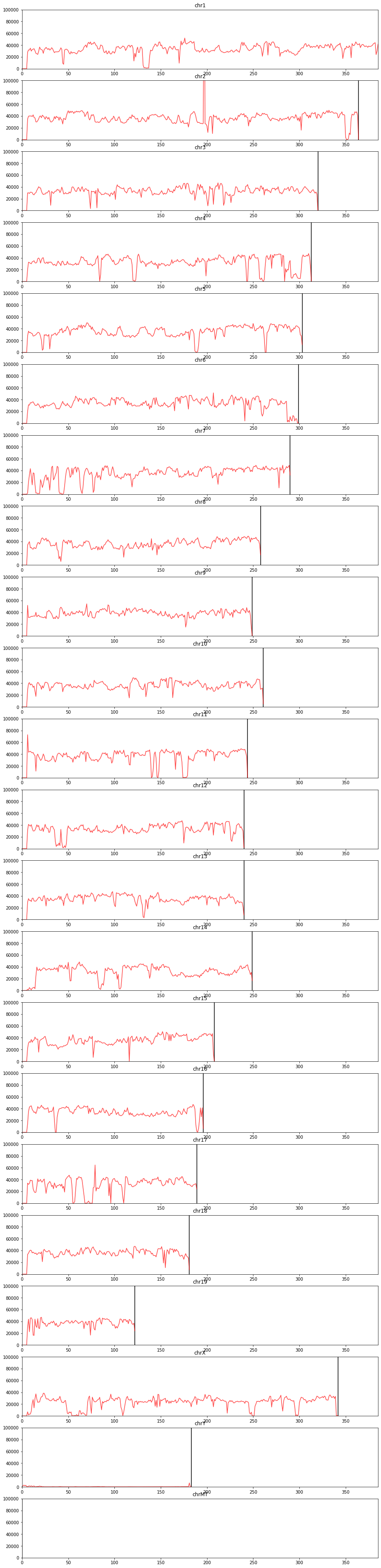
Note: decay by chromosome

With a bit of coding we can also extract the decay by chromosome.

Although the level of interaction changes depending on the chromosome (and the number of chromosomes, cf: chrX), the slope is relatively constant, and in very few occasions we may observe line crossings.

Differences in the slopes observed between chromosomes or conditions relates to gains or losses of close or long range interactions (Kojic et al. 2018).

from pytadbit import load_hic_data_from_reads
from matplotlib import pyplot as plt
import numpy as np

hic_data = load_hic_data_from_reads(reads, resolution=100000)

min_diff  = 1
max_diff  = 200

plt.figure(figsize=(12, 12))
for cnum, c in enumerate(hic_data.chromosomes):
    if c in ['chrY','chrMT']:
        continue
    dist_intr = []
    for diff in range(min_diff, min((max_diff, 1 + hic_data.chromosomes[c]))):
        beg, end = hic_data.section_pos[c]
        dist_intr.append([])
        for i in range(beg, end - diff):
            dist_intr[-1].append(hic_data[i, i + diff])
    mean_intrp = []
    for d in dist_intr:
        if len(d):
            mean_intrp.append(float(np.nansum(d)) / len(d))
        else:
            mean_intrp.append(0.0)
    xp, yp = range(min_diff, max_diff), mean_intrp
    x = []
    y = []
    for k in range(len(xp)):
        if yp[k]:
            x.append(xp[k])
            y.append(yp[k])
    l = plt.plot(x, y, '-', label=c, alpha=0.8)
    plt.hlines(mean_intrp[2], 3, 5.25 + np.exp(cnum / 4.3), color=l[0].get_color(),
               linestyle='--', alpha=0.5)
    plt.text(5.25 + np.exp(cnum / 4.3), mean_intrp[2], c, color=l[0].get_color())
    plt.plot(3, mean_intrp[2], '+', color=l[0].get_color())
plt.xscale('log')
plt.yscale('log')
plt.ylabel('number of interactions')
plt.xlabel('Distance between bins (in 100 kb bins)')
plt.grid()
plt.ylim(2, 250)
_ = plt.xlim(1, 110)

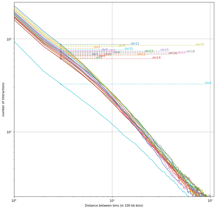
Note: thesedecay are computed on the raw data, and although the slopes may not change dramatically, it is agood practice to repeate this analysis and interpret the results also once the data are normalized.

In an ideal situation, the number of reads per bin along the genome is expected to be homogeneous across the genome. However, PCR artifacts (see for example the middle of the chromosome 3 below) or variations in the distributions of GC content, mappability or the number of RE cut-sites along the genome can cause heterogeneity. In the following sections, we will discuss how to correct for these sources of heterogeneity.

from pytadbit.mapping.analyze import plot_genomic_distribution

plot_genomic_distribution(reads, resolution=500000, ylim=(0, 100000), show=True)
plt.tight_layout()

<Figure size 432x288 with 0 Axes>

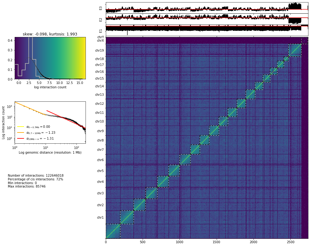
The plot bellow is probably the most informative, in order to infer the quality of an Hi-C experiment. This plot shows on the left part: - The histogram of the interaction counts. - The interaction count as a function of the genomic distance between the interacting sequences. - Some statistics on the specificity of the interaction: (i) the total number of interactions; (ii) the cis-to-trans ratio (expected to be at least between 50 or 60% in mammals), (iii and iv) the minimum and the maximum values of the ineraction matrix.

and on the right part:

• The interaction matrix.

• The first 3 eigenvectors of the interaction matrix are shown on top of the matrix itself.

Note: The first 3 eigenvectors of the interaction matrix highlight the principal structural features of the matrix. In the raw matrix shown here, we can see, for instance, that here the maxima of the first eigenvector seem to be correlated with the presence of low-coverage bins.

from pytadbit.mapping.analyze import hic_map

hic_map(reads, resolution=1000000, show=True, cmap='viridis')

From the reads that are mapped in a single RE fragment we can infer the average insert size:

from pytadbit.mapping.analyze import insert_sizes

insert_sizes(reads, show=True, nreads=1000000)

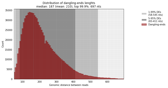
[187.0, 697.0]

The median size of the sequenced DNA fragments is thus 187 nt.

Note: This distribution is usually peaked at smaller values than the one measured experimentally (with a Bioanalyzer for example). This difference is due in part to the fact that, here, we are only measuring dangling-ends that may be, on average, shorter than other reads.

The following function in TADbit allows to measure the size of the sequenced fragment. If we set the parameter valid-pairs to False, we will look only at the interactions captured within RE fragments (similarly to the insert_sizes function above):

from pytadbit.mapping.analyze import  plot_strand_bias_by_distance

plot_strand_bias_by_distance(reads, valid_pairs=False, full_step=None, nreads=20000000)

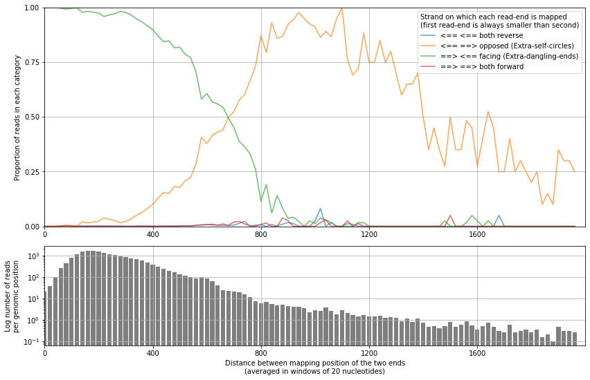
This function separates each read-end pair into 4 categories depending of the orientation of the strand in which each maps.

Having a look at the minimum distance from which the orientation of the mapped read-ends is even, is also useful for the interpretation of the results and for the definition of filters.

plot_strand_bias_by_distance(reads, nreads=20000000)

/home/dcastillo/miniconda2/envs/py3_tadbit/lib/python3.7/site-packages/pytadbit/mapping/analyze.py:1638: UserWarning: Attempted to set non-positive bottom ylim on a log-scaled axis.
Invalid limit will be ignored.
  axRb.set_ylim(0, max(sum_dirs) * 1.1)

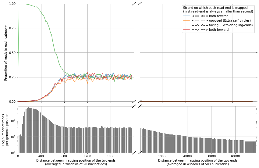
We can see that when the distance between the mapped read-ends is larger than ~1 kb, the orientation is even (25% each category). Meaning that bellow this size interactions are very likely to be extra-dangling-ends or re-ligated fragments, with no useful structural information.

References

[^](#ref-1) Mirny, Leonid a. 2011. The fractal globule as a model of chromatin architecture in the cell.. URL

[^](#ref-2) Aleksandar Kojic, Ana Cuadrado, Magali De Koninck, Daniel Giménez-Llorente, Miriam Rodríguez-Corsino, Gonzalo Gómez-López, François Le Dily, Marc A. Marti-Renom & Ana Losada. Distinct roles of cohesin-SA1 and cohesin-SA2 in 3D chromosome organization. Nature Structural & Molecular Biologyvolume 25, pages496–504 (2018) URL