Experimental data assessment and model parameters optimisation
Data preparation
The first step to generate three-dimensional (3D) models of a specific genomic regions is to filter columns with low counts and with no diagonal count in order to remove outliers or problematic columns from the interaction matrix. The particles associated with the filtered columns will be modelled, but will have no experimental data applied.
Here we load the data previous data already normalised.
from pytadbit import load_chromosome
from pytadbit.parsers.hic_parser import load_hic_data_from_bam
crm = load_chromosome('results/fragment/chr3.tdb')
B, PSC = crm.experiments
B, PSC
(Experiment mouse_B (resolution: 100 kb, TADs: 96, Hi-C rows: 1601, normalized: None),
 Experiment mouse_PSC (resolution: 100 kb, TADs: 118, Hi-C rows: 1601, normalized: None))
Load raw data matrices, and normalized matrices
base_path = 'results/fragment/{0}_both/03_filtering/valid_reads12_{0}.bam'
bias_path = 'results/fragment/{0}_both/04_normalizing/biases_{0}_both_{1}kb.biases'
reso = 100000
chrname = 'chr3'
cel1 = 'mouse_B'
cel2 = 'mouse_PSC'
hic_data1 = load_hic_data_from_bam(base_path.format(cel1),
                                   resolution=reso,
                                   region='chr3',
                                   biases=bias_path.format(cel1, reso // 1000),
                                   ncpus=8)
hic_data2 = load_hic_data_from_bam(base_path.format(cel2),
                                   resolution=reso,
                                   region='chr3',
                                   biases=bias_path.format(cel2, reso // 1000),
                                   ncpus=8)
(Matrix size 1601x1601)                                                      [2020-02-06 16:39:39]

- Parsing BAM (101 chunks)                                                   [2020-02-06 16:39:39]
   .......... .......... .......... .......... ..........     50/101
   .......... .......... .......... .......... ..........    100/101
   .                                                         101/101

- Getting matrices                                                           [2020-02-06 16:39:42]
   .......... .......... .......... .......... ..........     50/101
   .......... .......... .......... .......... ..........    100/101
   .                                                         101/101


(Matrix size 1601x1601)                                                      [2020-02-06 16:39:46]

- Parsing BAM (101 chunks)                                                   [2020-02-06 16:39:46]
   .......... .......... .......... .......... ..........     50/101
   .......... .......... .......... .......... ..........    100/101
   .                                                         101/101

- Getting matrices                                                           [2020-02-06 16:39:50]
   .......... .......... .......... .......... ..........     50/101
   .......... .......... .......... .......... ..........    100/101
   .                                                         101/101
B.load_hic_data([hic_data1.get_matrix(focus='chr3')])
B.load_norm_data([hic_data1.get_matrix(focus='chr3', normalized=True)])

PSC.load_hic_data([hic_data2.get_matrix(focus='chr3')])
PSC.load_norm_data([hic_data2.get_matrix(focus='chr3', normalized=True)])
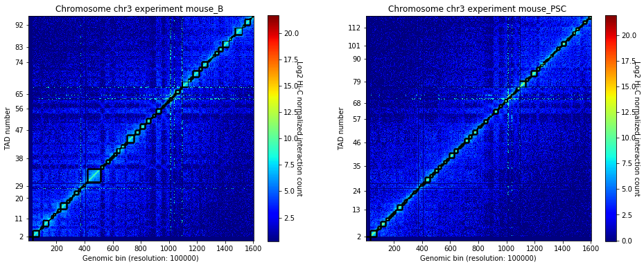
It is a good practice to check that the data is there:
crm.visualize(['mouse_B', 'mouse_PSC'], normalized=True, paint_tads=True)
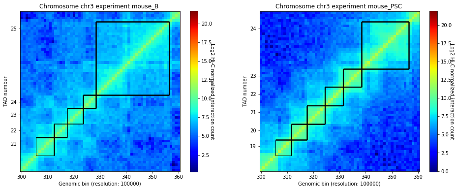
Focus on the genomic region to model.
crm.visualize(['mouse_B', 'mouse_PSC'], normalized=True, paint_tads=True, focus=(300, 360))
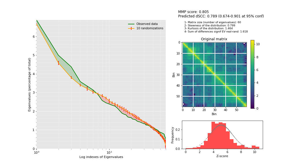
Data modellability assessment via MMP score
We can use the Matrix Modeling Potential (MMP) score (Trussart M. et al. Nature Communication, 2017) to identify a priori whether the interaction matrices have the potential of being use for modeling. The MMP score ranges from 0 to 1 and combines three different measures: the contribution of the significant eigenvectors, the skewness and the kurtosis of the distribution of Z-scores.
from pytadbit.utils.three_dim_stats import mmp_score
mmp_score(hic_data1.get_matrix(focus='chr3:30000000-36000000'),
          savefig='results/fragment/{0}_both/mmp_score.png'.format(cel1))
(0.8049308283731964,
 0.7885888244416531,
 0.6736346044021908,
 0.9006021702003049)
Data Transformation and scoring function
This step is automatically done in TADbit. A a weight is generated for each pair of interactions proportional to their interaction count as in formula:
The raw data are then multiplied by this weight. In the case that multiple experiments are used, the weighted interaction values are normalised using a factor (default set as 1) in order to compare between experiments. Then, a Z-score of the off-diagonal normalised/weighted interaction is calculated as in formula:
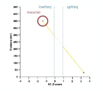
The Z-scores are then transformed to distance restraints. To define the type of restraints between each pair of particles. we need to identified empirically three optimal parameters (i) a maximal distance between two non-interacting particles (maxdist), (ii) a lower-bound cutoff to define particles that do not interact frequently (lowfreq) and (iii) an upper-bound cutoff to define particles that do interact frequently (upfreq). In TADbit this is done via a grid search approach.
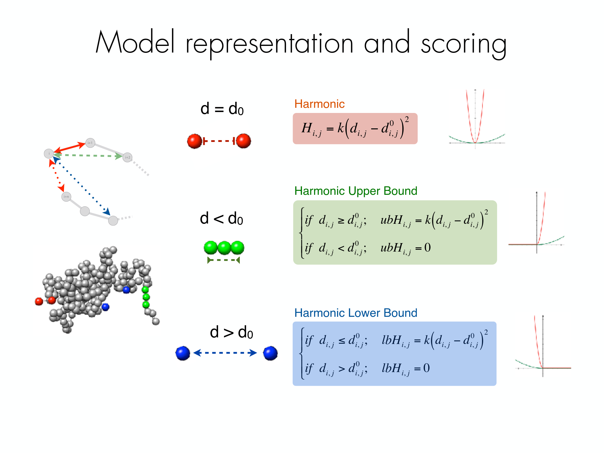
The following picture shows the different component of the scoring funtion that is optimised during the Monte Carlo simulated annealing sampling protocol. Two consecutive particles are spatially restrained by a harmonic oscillator with an equilibrium distance that corresponds to the sum of their radii. Non-consecutive particles with contact frequencies above the upper-bound cutoff are restrained by a harmonic oscillator at an equilibrium distance, while those below the lower-bound cutoff are maintained further than an equilibrium distance by a lower bound harmonic oscillator.
Optimization of parameters
We need to identified empirically (via a grid-search optimisation) the optimal parameters for the mdoelling procedure:
maxdist: maximal distance assosiated two interacting particles.
upfreq: to define particles that do interact frequently (defines attraction)
lowfreq: to define particles that do not interact frequently ( defines repulsion)
dcutoff: the definition of “contact” in units of bead diameter. Value of 2 means that a contact will occur when 2 beads are closer than 2 times their diameter. This will be used to compare 3D models with Hi-C interaction maps.
Pairs of beads interacting less than lowfreq (left dashed line) are penalized if they are closer than their assigned minimum distance (Harmonic lower bound). Pairs of beads interacting more than ufreq (right dashed line) are penalized if they are further apart than their assigned maximum distance (Harmonic upper bound). Pairs of beads which interaction fall in between lowfreq and upfreq are not penalized except if they are neighbours (Harmonic)
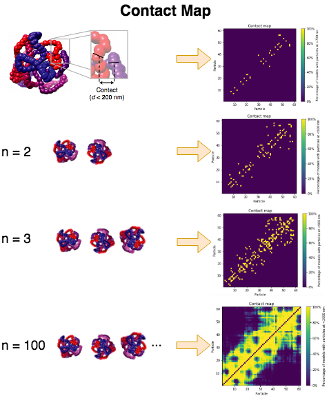
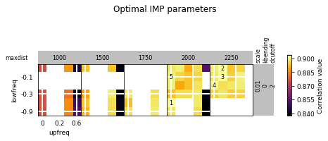
In the parameter optimization step we are going to give a set of ranges for the different search parameters. For each possible combination TADbit will produce a set of models.
In each individual model we consider that two beads are in contact if their distance in 3D space is lower than the specified distance cutoff. TADbit builds a cumulative contact map for each set of models as shown in the schema below. The contact map is then compared with the Hi-C interaction experiment by means of a Spearman correlation coefficient. The sets having higher correlation coefficients are those that best represents the original data.
opt_B = B.optimal_imp_parameters(start=300, end=360, n_models=40, n_keep=20, n_cpus=8,
                                   upfreq_range=(0, 0.6, 0.3),
                                   lowfreq_range=(-0.9, 0, 0.3),
                                   maxdist_range=(1000, 2000, 500),
                                   dcutoff_range=[2, 3, 4])
Optimizing 61 particles
  num scale kbending        maxdist lowfreq upfreq  dcutoff correlation
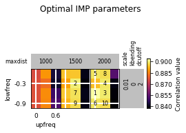
1   0.01  0               1000    -0.9    0       4      0.2021
1   0.01  0               1000    -0.9    0       3      0.5706
1   0.01  0               1000    -0.9    0       2      0.8769
2   0.01  0               1000    -0.9    0.3     4      0.3995
2   0.01  0               1000    -0.9    0.3     3      0.6799
2   0.01  0               1000    -0.9    0.3     2      0.8864
3   0.01  0               1000    -0.9    0.6     4      0.62
3   0.01  0               1000    -0.9    0.6     3      0.7709
3   0.01  0               1000    -0.9    0.6     2      0.8531
4   0.01  0               1000    -0.6    0       4      0.205
4   0.01  0               1000    -0.6    0       3      0.58
4   0.01  0               1000    -0.6    0       2      0.8773
5   0.01  0               1000    -0.6    0.3     4      0.4014
5   0.01  0               1000    -0.6    0.3     3      0.6827
5   0.01  0               1000    -0.6    0.3     2      0.8869
6   0.01  0               1000    -0.6    0.6     4      0.6181
6   0.01  0               1000    -0.6    0.6     3      0.776
6   0.01  0               1000    -0.6    0.6     2      0.8502
7   0.01  0               1000    -0.3    0       4      0.2084
7   0.01  0               1000    -0.3    0       3      0.5789
7   0.01  0               1000    -0.3    0       2      0.877
8   0.01  0               1000    -0.3    0.3     4      0.3999
8   0.01  0               1000    -0.3    0.3     3      0.6746
8   0.01  0               1000    -0.3    0.3     2      0.8824
9   0.01  0               1000    -0.3    0.6     4      0.6224
9   0.01  0               1000    -0.3    0.6     3      0.7678
9   0.01  0               1000    -0.3    0.6     2      0.8425
10  0.01  0               1000    0       0       4      0.19
10  0.01  0               1000    0       0       3      0.5669
10  0.01  0               1000    0       0       2      0.8763
11  0.01  0               1000    0       0.3     4      0.404
11  0.01  0               1000    0       0.3     3      0.6753
11  0.01  0               1000    0       0.3     2      0.8883
12  0.01  0               1000    0       0.6     4      0.6052
12  0.01  0               1000    0       0.6     3      0.7689
12  0.01  0               1000    0       0.6     2      0.8443
13  0.01  0               1500    -0.9    0       4      0.3574
13  0.01  0               1500    -0.9    0       3      0.6476
13  0.01  0               1500    -0.9    0       2      0.8926
14  0.01  0               1500    -0.9    0.3     4      0.4787
14  0.01  0               1500    -0.9    0.3     3      0.7314
14  0.01  0               1500    -0.9    0.3     2      0.8977
15  0.01  0               1500    -0.9    0.6     4      0.6623
15  0.01  0               1500    -0.9    0.6     3      0.7958
15  0.01  0               1500    -0.9    0.6     2      0.8401
16  0.01  0               1500    -0.6    0       4      0.3513
16  0.01  0               1500    -0.6    0       3      0.646
16  0.01  0               1500    -0.6    0       2      0.8951
17  0.01  0               1500    -0.6    0.3     4      0.4728
17  0.01  0               1500    -0.6    0.3     3      0.7341
17  0.01  0               1500    -0.6    0.3     2      0.8985
18  0.01  0               1500    -0.6    0.6     4      0.6491
18  0.01  0               1500    -0.6    0.6     3      0.7945
18  0.01  0               1500    -0.6    0.6     2      0.8407
19  0.01  0               1500    -0.3    0       4      0.367
19  0.01  0               1500    -0.3    0       3      0.6571
19  0.01  0               1500    -0.3    0       2      0.8897
20  0.01  0               1500    -0.3    0.3     4      0.4695
20  0.01  0               1500    -0.3    0.3     3      0.7355
20  0.01  0               1500    -0.3    0.3     2      0.9004
21  0.01  0               1500    -0.3    0.6     4      0.6568
21  0.01  0               1500    -0.3    0.6     3      0.7947
21  0.01  0               1500    -0.3    0.6     2      0.8391
22  0.01  0               1500    0       0       4      0.3722
22  0.01  0               1500    0       0       3      0.6566
22  0.01  0               1500    0       0       2      0.8943
23  0.01  0               1500    0       0.3     4      0.4745
23  0.01  0               1500    0       0.3     3      0.7278
23  0.01  0               1500    0       0.3     2      0.8946
24  0.01  0               1500    0       0.6     4      0.6529
24  0.01  0               1500    0       0.6     3      0.7951
24  0.01  0               1500    0       0.6     2      0.8404
25  0.01  0               2000    -0.9    0       4      0.4613
25  0.01  0               2000    -0.9    0       3      0.7304
25  0.01  0               2000    -0.9    0       2      0.8991
26  0.01  0               2000    -0.9    0.3     4      0.5551
26  0.01  0               2000    -0.9    0.3     3      0.7915
26  0.01  0               2000    -0.9    0.3     2      0.8977
27  0.01  0               2000    -0.9    0.6     4      0.6894
27  0.01  0               2000    -0.9    0.6     3      0.8012
27  0.01  0               2000    -0.9    0.6     2      0.8377
28  0.01  0               2000    -0.6    0       4      0.4717
28  0.01  0               2000    -0.6    0       3      0.7292
28  0.01  0               2000    -0.6    0       2      0.9036
29  0.01  0               2000    -0.6    0.3     4      0.5526
29  0.01  0               2000    -0.6    0.3     3      0.7815
29  0.01  0               2000    -0.6    0.3     2      0.8998
30  0.01  0               2000    -0.6    0.6     4      0.7032
30  0.01  0               2000    -0.6    0.6     3      0.8049
30  0.01  0               2000    -0.6    0.6     2      0.8387
31  0.01  0               2000    -0.3    0       4      0.4678
31  0.01  0               2000    -0.3    0       3      0.715
31  0.01  0               2000    -0.3    0       2      0.8939
32  0.01  0               2000    -0.3    0.3     4      0.5525
32  0.01  0               2000    -0.3    0.3     3      0.7861
32  0.01  0               2000    -0.3    0.3     2      0.8994
33  0.01  0               2000    -0.3    0.6     4      0.7005
33  0.01  0               2000    -0.3    0.6     3      0.804
33  0.01  0               2000    -0.3    0.6     2      0.8399
34  0.01  0               2000    0       0       4      0.4594
34  0.01  0               2000    0       0       3      0.7167
34  0.01  0               2000    0       0       2      0.8992
35  0.01  0               2000    0       0.3     4      0.5481
35  0.01  0               2000    0       0.3     3      0.7883
35  0.01  0               2000    0       0.3     2      0.8981
36  0.01  0               2000    0       0.6     4      0.692
36  0.01  0               2000    0       0.6     3      0.8032
36  0.01  0               2000    0       0.6     2      0.8541
opt_B.plot_2d(show_best=10)
Refine optimization in a small region:
opt_B.run_grid_search(upfreq_range=(0, 0.3, 0.3), lowfreq_range=(-0.9, -0.3, 0.3),
                       maxdist_range=[1750],
                       dcutoff_range=[2, 3],
                       n_cpus=8)
Optimizing 61 particles
  num scale kbending        maxdist lowfreq upfreq  dcutoff correlation
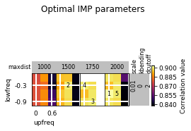
1   0.01  0               1750    -0.9    0       3      0.6859
1   0.01  0               1750    -0.9    0       2      0.8985
2   0.01  0               1750    -0.9    0.3     3      0.7587
2   0.01  0               1750    -0.9    0.3     2      0.9
3   0.01  0               1750    -0.6    0       3      0.6879
3   0.01  0               1750    -0.6    0       2      0.8937
4   0.01  0               1750    -0.6    0.3     3      0.7521
4   0.01  0               1750    -0.6    0.3     2      0.8993
5   0.01  0               1750    -0.3    0       3      0.6857
5   0.01  0               1750    -0.3    0       2      0.9
6   0.01  0               1750    -0.3    0.3     3      0.7644
6   0.01  0               1750    -0.3    0.3     2      0.8981
opt_B.plot_2d(show_best=5)
opt_B.run_grid_search(upfreq_range=(0, 0.3, 0.3), lowfreq_range=(-0.3, 0, 0.1),
                       maxdist_range=[2000, 2250],
                       dcutoff_range=[2],
                       n_cpus=8)
xx        0.01    0               2000    -0.3    0       4.0     0.4678
xx        0.01    0               2000    -0.3    0.3     4.0     0.5525
Optimizing 61 particles
  num scale kbending        maxdist lowfreq upfreq  dcutoff correlation
1   0.01  0               2000    -0.2    0       2      0.9001
2   0.01  0               2000    -0.2    0.3     2      0.8989
3   0.01  0               2000    -0.1    0       2      0.901
4   0.01  0               2000    -0.1    0.3     2      0.8967
xx        0.01    0               2000    0       0       4.0     0.4594
xx        0.01    0               2000    0       0.3     4.0     0.5481
5   0.01  0               2250    -0.3    0       2      0.8962
6   0.01  0               2250    -0.3    0.3     2      0.8964
7   0.01  0               2250    -0.2    0       2      0.9024
8   0.01  0               2250    -0.2    0.3     2      0.9004
9   0.01  0               2250    -0.1    0       2      0.8992
10  0.01  0               2250    -0.1    0.3     2      0.9009
11  0.01  0               2250    0       0       2      0.9001
12  0.01  0               2250    0       0.3     2      0.8967
opt_B.plot_2d(show_best=5)

opt_B.run_grid_search(upfreq_range=(0, 0.3, 0.1), lowfreq_range=(-0.3, 0, 0.1),
                       n_cpus=8,
                       maxdist_range=[2000, 2250],
                       dcutoff_range=[2])
xx 0.01 0 2000 -0.3 0 4.0 0.4678
Optimizing 61 particles
  num scale kbending        maxdist lowfreq upfreq  dcutoff correlation
1   0.01  0               2000    -0.3    0.1     2      0.898
2   0.01  0               2000    -0.3    0.2     2      0.8979
xx        0.01    0               2000    -0.3    0.3     4.0     0.5525
xx        0.01    0               2000    -0.2    0       2.0     0.9001
3   0.01  0               2000    -0.2    0.1     2      0.8908
4   0.01  0               2000    -0.2    0.2     2      0.8944
xx        0.01    0               2000    -0.2    0.3     2.0     0.8989
xx        0.01    0               2000    -0.1    0       2.0     0.901
5   0.01  0               2000    -0.1    0.1     2      0.8967
6   0.01  0               2000    -0.1    0.2     2      0.8941
xx        0.01    0               2000    -0.1    0.3     2.0     0.8967
xx        0.01    0               2000    0       0       4.0     0.4594
7   0.01  0               2000    0       0.1     2      0.9006
8   0.01  0               2000    0       0.2     2      0.8914
xx        0.01    0               2000    0       0.3     4.0     0.5481
xx        0.01    0               2250    -0.3    0       2.0     0.8962
9   0.01  0               2250    -0.3    0.1     2      0.8991
10  0.01  0               2250    -0.3    0.2     2      0.8957
xx        0.01    0               2250    -0.3    0.3     2.0     0.8964
xx        0.01    0               2250    -0.2    0       2.0     0.9024
11  0.01  0               2250    -0.2    0.1     2      0.8984
12  0.01  0               2250    -0.2    0.2     2      0.8993
xx        0.01    0               2250    -0.2    0.3     2.0     0.9004
xx        0.01    0               2250    -0.1    0       2.0     0.8992
13  0.01  0               2250    -0.1    0.1     2      0.9024
14  0.01  0               2250    -0.1    0.2     2      0.8959
xx        0.01    0               2250    -0.1    0.3     2.0     0.9009
xx        0.01    0               2250    0       0       2.0     0.9001
15  0.01  0               2250    0       0.1     2      0.9033
16  0.01  0               2250    0       0.2     2      0.895
xx        0.01    0               2250    0       0.3     2.0     0.8967
opt_B.plot_2d(show_best=5)
opt_B.get_best_parameters_dict()
{'scale': 0.01,
 'kbending': 0.0,
 'maxdist': 2000.0,
 'lowfreq': -0.6,
 'upfreq': 0.0,
 'dcutoff': 2.0,
 'reference': '',
 'kforce': 5}
For the other replicate, we can reduce the space of search:
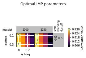
opt_PSC = PSC.optimal_imp_parameters(start=300, end=360, n_models=40, n_keep=20, n_cpus=8,
                                     upfreq_range=(0, 0.3, 0.1),
                                     lowfreq_range=(-0.3, -0.1, 0.1),
                                     maxdist_range=(2000, 2250, 250),
                                     dcutoff_range=[2])
Optimizing 61 particles
  num scale kbending        maxdist lowfreq upfreq  dcutoff correlation
1   0.01  0               2000    -0.3    0       2      0.9309
2   0.01  0               2000    -0.3    0.1     2      0.9237
3   0.01  0               2000    -0.3    0.2     2      0.9177
4   0.01  0               2000    -0.3    0.3     2      0.9084
5   0.01  0               2000    -0.2    0       2      0.9268
6   0.01  0               2000    -0.2    0.1     2      0.9245
7   0.01  0               2000    -0.2    0.2     2      0.9159
8   0.01  0               2000    -0.2    0.3     2      0.9095
9   0.01  0               2000    -0.1    0       2      0.9283
10  0.01  0               2000    -0.1    0.1     2      0.9239
11  0.01  0               2000    -0.1    0.2     2      0.9136
12  0.01  0               2000    -0.1    0.3     2      0.9071
13  0.01  0               2250    -0.3    0       2      0.9285
14  0.01  0               2250    -0.3    0.1     2      0.9233
15  0.01  0               2250    -0.3    0.2     2      0.9165
16  0.01  0               2250    -0.3    0.3     2      0.9068
17  0.01  0               2250    -0.2    0       2      0.9294
18  0.01  0               2250    -0.2    0.1     2      0.9214
19  0.01  0               2250    -0.2    0.2     2      0.9154
20  0.01  0               2250    -0.2    0.3     2      0.9041
21  0.01  0               2250    -0.1    0       2      0.9304
22  0.01  0               2250    -0.1    0.1     2      0.9219
23  0.01  0               2250    -0.1    0.2     2      0.9157
24  0.01  0               2250    -0.1    0.3     2      0.9076
opt_PSC.plot_2d(show_best=5)
opt_PSC.get_best_parameters_dict()
{'scale': 0.01,
 'kbending': 0.0,
 'maxdist': 2000.0,
 'lowfreq': -0.3,
 'upfreq': 0.0,
 'dcutoff': 2.0,
 'reference': '',
 'kforce': 5}
